�

Semiconductor Components Industries, LLC, 2003

October, 2003 - Rev. 1

Publication Order Number:

AND8112/D

AND8112/D

A Quasi-Resonant SPICE
Model Eases Feedback
Loop Designs

Prepared by: Christophe Basso

Prepared by:

Joel Turchi

ON Semiconductor

Within the wide family of Switch Mode Power Supplies

(SMPS), the Flyback converters represent the structure of
choice for use in small and medium power applications. For
compact designs and radio-frequency sensitive
applications,

e.g. TV sets or set-top boxes, Quasi- Resonant

power supplies start to take a significant market share over
the traditional fixed frequency topology. However, if the
feedback loop control is well understood with this latter, for
instance via a comprehensive literature and SPICE models,
the situation differs for self-oscillating variable switching
frequency structures where no model still exists. This article
will show how a simple large-signal averaged SPICE model
can be derived and used to ease the design work during
stability analysis.

Quasi-Resonant Operation

It is difficult to abruptly dig into the analytical analysis

without giving a basic idea of the operation of a converter
working in Quasi-Resonance (QR). Figure 1 depicts a
typical FLYBACK converter drain-source waveform as you
probably have already observed. When the switch is closed,
the drain-source voltage V

is near 0 V and the input

voltage V

appears across the primary inductance L

: the

current inside L

ramps up with a slope of

SON

Vg
LP

(eq. 1)

When the controller instructs the switch opening, the

drain-source quickly rises and the energy transfer between
primary and secondary takes place: the secondary diode
conducts and the output voltage flies back on the primary
side, over L

. This "Flyback" plateau is equal to V

+ (V +

) / N, where N is the secondary to primary turn ratio, V the

output voltage and V

the diode forward voltage drop.

During this time, the primary current decreases with a slope
now imposed by the reflected voltage

SOFF

)

Vf)

(eq. 2)

Figure 2 zooms on the simulated primary current (actually

circulating in the magnetizing inductor), showing how it
moves over one switching cycle.

OFF

Figure 1. A Typical FLYBACK Drain-Source

Waveform

Core is Reset

Valleys

Plateau:

out

+ V

)/N

Leakage Inductance

OFF

Figure 2. The Primary Current Ramps Up and Down

to Zero in DCM

peak

= V

= 0, Reset

off

= (V + V

) / (L

x N)

When the primary current reaches zero, the transformer

core is fully demagnetized: we are in Discontinuous
Conduction Mode (DCM). The primary inductance L

together with all the surrounding capacitive elements C

tot

create a LC filter. When the secondary diode stops conducting
at I

= 0, the drain branch is left floating since the MOSFET

is already open. As a result, a natural oscillation occurs,
exhibiting the following frequency value:

Fring

@ p @

Ctot

(eq. 3)

http://onsemi.com

AND8112/D

http://onsemi.com

As in any sinusoidal signal, there are peaks and valleys. When you re-start the switch in one valley, where the voltage is

minimum, the MOSFET is no longer the seat of heavy turn-on losses engendered by capacitive effects: this is the so-called
Quasi-Resonance operation where the switching frequency depends on the peak current, the various slopes ON and OFF and
the number of valleys you choose after the core reset. In our study, we will first concentrate on a simplified SPICE version where
the power switch is actuated right after the reset detection point (parasitic ringings are neglected) and later on, a more
sophisticated declination will incorporate parasitic delays.

Modeling the Switch Network

Figure 3 depicts a Flyback topology where the switching

elements generating the above waveforms have been
highlighted: the power switch (usually a MOSFET
transistor) and a diode, performing a rectification job.
During the converter operation, the Pulse Width Modulator
controller (PWM) instructs the transistor to turn ON, in
order to store energy in the primary side. The primary
current builds up until the setpoint imposed by the feedback
loop is reached. At this time, the controller toggles the
transistor to the OFF state and energy transfers to the
secondary side. If the ON and OFF states can be described
by a set of linear equations, there exists a discontinuity
linking these two events. Despite the presence of linear
elements in the converter (capacitors, inductors and
resistors), the presence of the commuting switch clearly
introduces the non-linearity that prevents us from directly
writing the small-signal equations

...

When learning electronic circuits at school, there were

some exercises in which we were asked to reveal the transfer
function of bipolar amplifiers. At that time, we learned to
replace the transistor symbol by its equivalent small-signal
model: the schematic turned into the simple association of
current and voltage sources that greatly simplified the
analysis. In the average circuit modeling technique, we also
follow the same philosophy: the exercise lies in isolating and
replacing the switch network with a set of current and
voltage sources whose electrical architecture do not vary
with time. Therefore, plugging the equivalent model back
into the converter of interest allows us to resolve its transfer
characteristics.

Figure 3. A Flyback Power Supply where Switches

have been Isolated

(t)

2(t)

1(t)

Control

1(t)

L(t)

1:N

Figure 4.

and Individual Signals Separately Plotted.

(V(L

)

V
N

2(t)

1(t)

2(t)

1(t)

L(t)

V
N

)

Vg
LP

)

Deriving Equations

The object of deriving a model consists in writing the

equations that describe the switch network averaged input
and output quantities that a) depend from each other b) obey
to the control input. Let us draw the various waveforms
before starting any line of algebra (Figure 4). From this
picture, we can develop equations that will finally describe
the averaged evolution of the values of interest, the input /
output voltage and current of our switch network:

I1(t)

(eq. 4)

I2(t)

(eq. 5)

V1(t)

)

(eq. 6)

V2(t)

)

Vg]

(eq. 7)

where: V is the output voltage, V

the input voltage, I

the

primary peak current, N the N

/ N

turn ratio and d the

duty-cycle (d

= 1 �d).

Please note that in this first approach, we do not consider

any delay occurring at the switch opening or induced by
equation 3. These events will considered later on, in a more
complex model.

AND8112/D

http://onsemi.com

Averaging Input / Output Voltages

From the inductor volt-second balance approximation, we know that the average voltage across an inductor operated in a

steady-state converter is null. By looking at the V(L

) sketch, we obtain the following equation:

V(LP)

d(t)

Vg(t)

u *

d (t)

V(t)

(eq. 8)

d(t)

Vg(t)

u *

d(t))

V(t)

which lets us extract the classical output / input voltage ratio

V(t)

Vg(t)

u +

d(t)

d(t))

(eq. 9)

and as a result, the duty-cycle expression:

d(t)

V(t)

u )

Vg(t)

(eq. 10)

Now, by plugging equation 10 in equation 6, we obtain the average voltage across the primary switch terminal: <V

1(t)

> =

V(t)

u )

Vg(t)

d(t))

V(t)

u )

Vg(t)

V(t)

u )

Vg(t)

u +t

Vg(t)

(eq. 11)

which agrees with the inductor volt-second balance approximation (from Figure 1 since, by definition, <V(L

)> = 0, then V

appears across the switch terminals).

To reveal <V

2(t)

>, let us plug equation 10 into 7: <V

2(t)

> =

[

V(t)

u )

Vg(t)

]

d(t)

[

V(t)

u )

Vg(t)

]

V(t)

u )

Vg(t)

u +t

V(t)

(eq. 12)

which again could be deduced from Figure 3 since the average voltage across the secondary inductance is zero

...

Averaging Input / Output Currents

The peak inductor current depends on the time during

which V

is applied over L

. If we recall that this time

(actually t

) is d x T

, then:

Vg
LP

(eq. 13)

From Figure 4, the average current <I

1(t)

> can be obtained

by evaluating the triangular area (charge in Coul

omb

) and

dividing by the switching period. This is expressed by
equation 4. Now plugging equation 13 in 4, we obtain:

I1(t)

1
2

Vg(t)

d(t)

(eq. 14)

Vg(t)

d(t)

however, from equation 11, we know that <V

1(t)

> = <V

g(t)

thus equation 14 turns into:

I1(t)

V1(t)

d(t)

(eq. 15)

Applying the same technique to the secondary current

2(t)

, leads to:

I2(t)

d.TS

I2(t)

1
2

d (t)

(eq. 16)

plugging equation 13 in 16 leads to:

I2(t)

Vg(t)

d(t)

d(t))

(eq. 17)

V1(t)

d(t)

d(t))

A 100% Efficiency Power Transfer

...

Assuming that 100% of the primary stored energy is

released to the secondary side, then we can use equations 11
and 12 to write:

(eq. 18)

(t)

> = <V

1(t)

> X <I

1(t)

> = <V

2(t)

> X <I

2(t)

From equation 15, we can see that a current is generated

by a voltage multiplied by a term. This term is obviously
homogenous to the inverse of an impedance. By
re-arranging equation 15, we obtain:

AND8112/D

http://onsemi.com

Re(d)

V1(t)

I1(t)

u +

d(t)

(eq. 19)

where the input impedance depends on the duty-cycle d

(t)

However, in quasi-resonant converters, the power transfer
adjusts by varying the peak current I

which finally imposes

the operating frequency. Since by definition t

= d x T

, we

can re-arrange equation 9 to reveal

ton

Vg)

)

(eq. 20)

By finally plugging equation 10 and 20 into 19, we obtain

a t

-dependent input effective resistance definition:

Re(ton)

)

Vg)

ton

(eq. 21)

that Figure 5 portrays:

The average input waveforms of the switch can be modeled via

the above equivalent network.

Figure 5.

1(t)

Re(t

)

The two-port loss-free network where all the input power trans-

forms into output power.

Figure 6.

1(t)

Re(t

)

(t)

2(t)

As reference [1] details, the apparent power consumed by

, P

, is entirely transmitted to the output since we assume

a 100% efficiency. Therefore, equation 19 can be re-written
by:

P(t)

u+t

V1(t)

u t

I1(t)

(eq. 22)

V2(t)

u t

I2(t)

V1(t)

Re(ton)

Our switch network can thus modeled according to the

so-called loss-free network where all the power developed
across an input resistance transfers to the output without any
loss (Figure 6) [1].

A More Complex Model Including Parasitic Effects

The above simplified model assumes that there are no

transient times between the conduction and
demagnetization phases. A more precise modelling
approach requires that the two following delays

and

are taken into account, as highlighted by Figure 7 and 8:

Figure 7.

The presence of a capacitive node slows-down the V

rising

and makes the drain sinusoidally ring at the core reset

...

Core Is Reset!

1. At the end of the ON-time, the power switch

opens but the energy transfer to the secondary side
does not start immediately. The primary inductor
current (I

) that cannot flow through the power

switch, charges the surrounding capacitive
elements (C

tot

) until C

tot

voltage exceeds

)

V
N

(eq. 23)

At that moment, the secondary diode starts to
conduct and current feeds the output capacitor. One
can assume that the C

tot

charging time (

) is short

enough to consider that the primary inductor current
stays equal to I

during this interval. Then,

is the

time necessary to charge the capacitor C

tot

with a

current I

from zero to

)

V
N

(eq. 24)

Ctot

)

V
N

, i.e.:

AND8112/D

http://onsemi.com

NCP1207

Figure 8.

tot

out

<=>

When the power switch turns off, the primary inductor behaves like a current source that charges the C

tot

capacitor. This sequence ends

when voltage developed across C

tot

exceeds [V

+(V+V

)/N], that is when the secondary diode D1 starts to conduct.

2. At the end of the core reset, both switches (power

switch and secondary diode) are off. The primary
inductor L

together with C

tot

form a LC network.

tot

voltage (and thus the drain source voltage of

the power switch) oscillates around the input
voltage V

between a peak value (the initial level:

)

V
N

) and a valley value

V
N

the damping

effects being neglected. To benefit from the quasi-
resonant mode, it is recommended to turn the power
switch on in the valley, where the drain-source
voltage is minimized. This naturally reduces the
dV/dt and switching losses to a minimum (in
practice, an appropriate delay inserted after the core
reset detection provides an effective method to
synchronize the power switch turn on with the valley
event). A simple look at Figure 7 shows that the
valley occurs at half the oscillation period.
Therefore, the delay

between the core reset

completion and the optimal turn on time is given by
the following equation:

+ p

Ctot

(eq. 25)

Once these delays are defined, it is about time to revise the

previous equations in order to include

and

effects.

The main parameters of interest are the average input and
output currents, the equivalent resistance and the switching
period. If we combine equations 24 and 13 that express I

a function of the input voltage, the inductor value and the
ON-time leads to:

Ctot

)

V
N

ton

(eq. 26)

If (d

x T

) depicts the core reset time,

and

times

require to change (d

=1-d) into:

) D

(eq. 27)

The inductor volt-second balance approximation of

equation 8 still holds. However, it must be revised by

replacing d

(t) by its novel value as expressed by

equation (27):

V(LP)

(eq. 28)

Re-arranging equation (28), one can unveil the duty cycle

expression:

Vg)

)

(eq. 29)

The switching period is the sum of the on-time, the core

reset time (t

demag

and

ton

)

tdemag

) D

(eq. 30)

The time t

demag

can be easily deducted from the Figure 4

sketch. Since the core reset is the time necessary to discharge
the primary inductor from I

to zero with a (V+V

)/N slope,

it comes:

tdemag

V N

ton

(eq. 31)

Substitution of equation (31) into (eq. 30), leads to the

following expression where T

is a function of t

+ D

) D

)

[(N

Vg)

)

ton

(eq. 32)

Equation (15) that defines the average input current as a

function of the input voltage, the duty cycle, the inductor
value and the switching period, still holds. Substitution of
equation (29) into equation (15) leads to:

I1(t)

ton

[(N

Vg)

)

(eq. 33)

Replacing T

by its equation 32 expression, it comes:

I1(t)

)

Vg)

)

ton

[(N

Vg)

)

(eq. 34)

Re-arranging this equation, one can obtain:

AND8112/D

http://onsemi.com

I1(t)

ton

) D

)

Vg)

)

ton

(eq. 35)

Similarly to the simplified model analysis, one can note

that the average input current is proportional to the input
voltage. The effective resistance Re is thus: Re(t

) =

ton

) D

)

[(N

Vg)

)

ton

(eq. 36)

It is pleasant to confirm that if

=0, the Re(t

)

expression reduces to equation 21

...

Then, the equivalent circuit depicted in Figure 6 and based

on the loss-free resistor Re(t

) can be applied. To complete

the model, let's calculate <I

2(t)

> by combining equations

(17) where d

is taken equal to (t

demag

), (13) and (31):

I2(t)

ton

(eq. 37)

Substitution of equation (32) giving T

into equation (37),

leads to: <I

2(t)

> =

ton

) D

)

Vg)

)

ton

(eq. 38)

This expression can be simplified as follows: <I

2(t)

> =

Re(ton)

)

I1(t)

)

(eq. 39)

The model assumes a 100% efficiency power transfer. To

better stick to reality, the above expression should be
multiplied by the estimated efficiency to obtain the final
<I

2(t)

> equation:

I2(t)

u+t

I1(t)

)

eff

(eq. 40)

where eff is the efficiency.

AND8112/D

http://onsemi.com

The following table summarizes the main equations upon which our model is based:

Delay between the power switch opening and the start of the ener-
gy transfer to secondary side:

Ctot

)

V
N

ton

Delay between the core reset completion and the next turn on of
the power switch (Note 1):

+ p

Ctot

Equivalent input resistance:

Re(ton)

ton

) D

)

[(N

Vg)

)

ton

Switching Frequency:

fSW

) D

)

Vg)

)

ton

Average input current:

I1(t)

Vg Re(ton)

Average output current:

I2(t)

I1(t)

u eff

NOTE:

: even if the proposed value appears to us as the
optimal one, SMPS designers might make a
different choice for

. That is why, if the model

proposes

+ p

Ctot

as default

value, you can modify this simulation parameter
to stick to your application in case valley
switching is not considered.

Implementing the SPICE Model with the
Loss-Free Network

As exemplified by Figure 6, the model shall emulate an

input resistor being t

dependent and then transmit a power

following equation 23. Different ways exist to implement
this topology in Spice. INTUSOFT's IsSpice authorizes
behavioral resistors, e.g. following any particular ohmic
evolution with time, voltage, current etc. For instance, the
following code would be accepted by the simulator:

R1 1 2 R = 2.0 * v(1)^0.5 + 3.0*v(2)*time + v(2)*sqrt(temp)

Unfortunately, despite its obvious interest, this code is not

very portable and would constrain the model usage to
IsSpice only. Figure 9 offers a more practical association
using behavioral voltage and current sources [2]:

Figure 9. Implementing the DCM Model via Two

Controlled Elements

The input voltage source being supposed to emulate a

resistance, its expression shall be in the form of:

Et = I

x Re where Re is simply equation 22, thus:

)

Vg)

ton

(eq. 41)

where t

is an input port of the model, imposed by the

control loop. In the final model, this value will be derived
from L

and the peak current given by the error voltage

divided by R

sense

, where V, V

and N are to be passed or

sensed by the model.

The output current source together with V

shall deliver

the output power as imposed by equation 22. Thus, i

generation shall follow:

Rin(eq)

)

Vg)

ton

(eq. 42)

Also, one can introduce the efficiency by simply

multiplying the I

current source by {eff}, where eff is a

parameter entered by the user in the model. Hence, I

can be

written as:

)

Vg)

ton

eff

(eq. 43)

AND8112/D

http://onsemi.com

BEt
Voltage

VI1

(2*{Lp}*(V(3)+{N}*V(13))/(V(ton)*V(3)+1u))*I(V6)

BGd
Current

(((2*{Lp}*(V(3)+{N}*V(13))/(V(ton)*V(3)+1u))*I(V6)^2)/(V(3,4)+1u))*{eff}

Bton
Voltage
V(errint)*{Lp}/({Rs}*V(13))

{Rlf}

X2
XFMR
RATIO = N

Lm
{Lp}

R9
1 Meg

BIp
Voltage
V(ton)*V(13)/{Lp}

BToff
Voltage
{Lp}*V(Ip)*{N}/V(3)

Bfreq

Voltage

(1/(V(ton)+V(toff)))/1 k

Bclamp
Current

I(VI1)>0 ?
I(VI1) :
0

System Parameter calculation

Operating Parameter Calculation

B8
Voltage
V(FB)/3 > 1 ? 1 : V(FB)/3 < 10 m
? 10m : V(FB)/3

errint

Gnd

Figure 10. The final simplified model implementation where added sources reveal operating parameters

such as T

, F

and the peak current I

off

Figure 10 portrays the final simplified model subcircuit where all relevant sources appear, among them, the switching

frequency, peak current and T

calculations. For the extended model, only BGd and BEt sources need to be changed. As you

can see, there are plenty denominator expressions where a variable such as T

appears. If during the bias point calculation

SPICE T

starts or goes close to zero, the simulator can fail to converge (or find a wrong bias point which is worse). To avoid

this potential problem, a trick consists in inserting a fixed value, small enough like 1

m or less, to clamp the maximum value

the source can take if T

becomes null. To the opposite, the frequency expression modeled by a voltage source can deliver

kV to express kilo Hz. The simulator dynamic being bounded, mixing values of a few mV with sources delivering kV can puzzle
the bias point calculation. Again, a division by 1000 will limit the range. The FB pin undergoes a division by 3 to be further
clamp by a 1 V limiter, a classical circuitry found in most PWM controllers (I

max = 1 V / R

sense

DC-bias calculation always represents a difficult task for SPICE simulators running averaged models. In order to enhance

the extended model robustness (the one including parasitic effects), we have constrained the BGd source to be positive only
by using a simple in-line equation that differs depending on the simulator syntax:

IsSpice

BGd 4 3 I= ((2*{Lp}/V(ton)) * ( ({N}*V(13)+V(3))/(V(3)+1u) + {DEL}/V(ton) +
+({Lp}*{Ctot}/V(ton))*(1+(V(3)/{N})/V(13)) ) * I(V6)^2)/(V(3,4)+1u)*{EFF} < 10m ? 10m :
+((2*{Lp}/V(ton)) * ( ({N}*V(13)+V(3))/(V(3)+1u) + {DEL}/V(ton) +
+({Lp}*{Ctot}/V(ton))*(1+(V(3)/{N})/V(13)) ) * I(V6)^2)/(V(3,4)+1u)*{EFF}

PSpice

Gd 4 3 TABLE { ((2*{Lp}/(V(ton)+10n)) * ( ({N}*V(13)+V(3))/(V(3)+1u) + {DEL}/(V(ton)+10n) +
+({Lp}*{Ctot}/(V(ton)+10 n))*(1+(V(3)/{N})/V(13)) )
+ * I(V6)^2)/(V(3,4) + 1u)*{EFF} } ( (10m,10m) (1000,1000) )

Finally, the model comes with two different names:

.SUBCKT QuasiFly 13 FB GND 3 I

params: L

= 3.22 m R

= 0.5 N = 0.06 eff = 0.86

the simplified model version
QuasiFlyDel 13 FB GND 3 I

params: L

= 3.22 m R

= 0.8 N = 0.06 eff = 0.86 C

tot

= 100 p

the complete model including parasitic effects

Passed parameters are:

tot

, the lump parasitic component present on the drain.

, the primary inductance

, the ohmic losses of the primary winding

N, the N

: N

ratio with N

Eff, the circuit estimated efficiency

Please note that for the sake of simplicity, both models do not account for the secondary rectifier forward drop V

whose effect

is nevertheless negligible in our approach.

AND8112/D

http://onsemi.com

Putting the Model to Work

Different ways exist to test the validity of a model. The

first one is by using SPICE only, where one can compare the
transient response of the averaged model versus that of the
equivalent cycle-by-cycle. The other one implies the
comparison of the averaged model results versus a real board
measurement. In this paper, we will depict both approaches,
using our simplified cycle-by-cycle transient model.

The averaged template is depicted by Figure 11 where

Figure 10 sources have been pushed into a single graphic

symbol. The symbol must be fed by Lp, Efficiency, R

sense

transformer turn ratio and the primary inductance ohmic
loss. The FB pin goes to a component arrangement particular
to the NCP1207 series from ON Semiconductor where the
optocoupler collector is internally pulled-up to a reference
voltage.

60 m

1 k

D4
BV = 15.6

1 n

10 m

150 m

R10

20 k

4.8

Flyback FreeRunning

Averaged model

GND

OUT

X1
SFH615AGR

120

16.8

16.7

15.8

1.30

16.8

4.80

Figure 11. Averaged Model Template

out

load

8.5

C4
220

C3
1 mF
I

= 16

2.2

X2
QuasiFly
L

= 1.2 m

= 0.5

N = 0.06
eff = 0.91
Rlf = 0.5

120
AC =

0.868

8.68

80.7
f

(kHz)

The averaged model template featuring DC bias points which confirms the correct bias point calculation

In Figure 11, once the simulation has been done, DC

points are reflected to the schematic and confirm the validity
of the original calculation. The feedback loop is made of a
simple Zener diode to avoid any long feedback time
constants as with a standard TL431. The cycle-by-cycle
circuitry uses our simplified QR transient model which
emulates a free-running controller such as
ON Semiconductor NCP1207 or NCP1205 [3] (Figure 12).
The output stage and feedback configuration conforms to
Figure 11 in order to compare similar topologies. The first
test consists in testing the input audio susceptibility by
stepping the input voltage from 200 V to 350 VDC.

Figure 13 reveals the good agreement between the averaged
response and the cycle-by-cycle one. The next experience
will step load the converter output from light to heavy load
in a few

ms. Figure 14 testifies for the right behavior on both

configuration, average or cycle-by-cycle.

On the static point of view, the following data compare

numbers given by the averaged model and the
cycle-by-cycle one:

AVG = 868 mA / I

TRAN = 858 mA

AVG = 8.68

ms / T

TRAN = 8.78

AVG = 80.7 kHz / F

AVG = 77.8 kHz

AND8112/D

http://onsemi.com

1 k

dem

Resr1
60 m

X4
XFMR-AUX
RATIO_POW = -0.06
RATIO_AUX = -0.06

D4
BV = 15.6

dem

Feedback

100

100 p

X2
PSW1

FreeRun

FreeRunDT

10 m

R7
150 m

MBR20100CT

X5
SFH615AGR

V3
120
AC =

Simplified simulation of a
NCP1207-based board

X3
PSW1

Figure 12. This Simplified Transient Model Will Help to Check the Averaged Results

leak

1 p

prim

0.5

Coil

1 n

out

led

1 k

drain

reso

10 p

Reso

coil

prim

1.2 m

out1

1 mF
I

= 16.5

sense

0.5

off(min)

= 1

out

Diode

2.2

C1
220

= 16.5

2.57 m

3.11 m

3.65 m

4.19 m

4.73 m

16.80

16.82

16.84

16.86

16.88

Figure 13. Audio Susceptibility with a Line Step

(200 to 350 V)

Cycle-by-Cycle V

out

Averaged V

out

Figure 14.

and Load Step Response

Comparison Between Models (50

to 0.5

)

2.48 m

3.04 m

3.60 m

4.16 m

4.72 m

16.55

16.65

16.75

16.85

16.95

Cycle-by-Cycle V

out

= 20 mV

Averaged V

out

Real World Confrontation

Even if the above paragraph gives us the assumption that

our model sticks to reality quite well, nothing replaces a real
board measurement with a network analyzer. However, on
the NCP1207, the collector of the optocoupler is directly
internally pulled-up to a reference via a resistor, it thus
becomes difficult to open the loop via the series transformer
method. We thus went back to a simple open-loop
configuration where a DC source fixes the expected
operating point. It does not cause any problem in our case
since the overall gain V

control

to V

out

is low. The AC

injection is then made via a 1000

mF capacitor. Figure 15

depicts the adopted configuration on the bench, but also
replicated on the averaged model.

NCP1207

Figure 15.

sense

R3
1 k

bias

1.57

stim

AC = 1

1000

The AC measurement is obtained once the proper

operating point is reached by adjusting V

bias

. The gain being

low, there is no problem of output runaway as long as V

bias

is slowly increased.

AND8112/D

http://onsemi.com

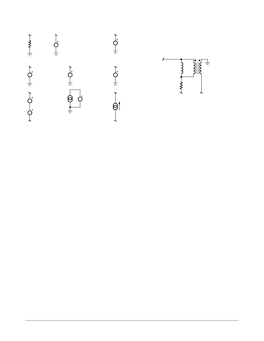
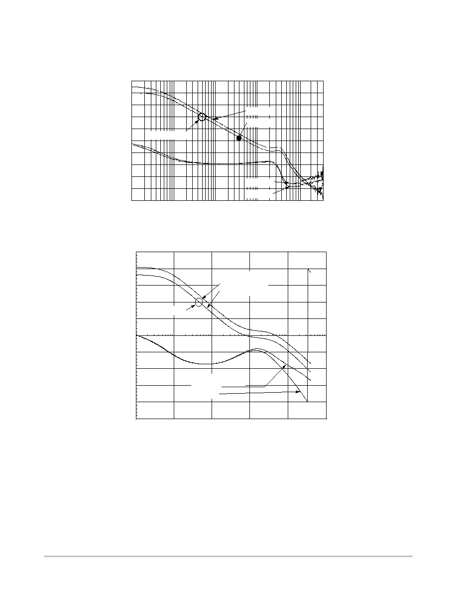
The bandwidth measurement has been carried on a board further to a 15 mn warm-up. This board does not use any clamping

network but a 800 V MOSFET instead and a large capacitor connected between drain and ground Figure 16 and 17 compare
the obtained results with the averaged model including valley and turn-off delays:

100

1 k

10 k

100 k

-180

-90.0

90.0

180

-60.0

-40.0

-20.0

20.0

Figure 16. Bode Plot Captured with a Network Analyzer

Figure 17. Bode Plot Obtained with the Averaged Model

Open-loop Phase:
High Line
Low Line

Open-loop Gain:
High Line
Low Line

F0 dB = 46 Hz

10 k

1 k

100

-10

-20

-30

-40

-50

-60

Mag (dB)

180

Phase (

�

)

135

-45

-90

-135

-180

F0 dB = 49 Hz

High Line

Low Line

High Line

Low Line

One can detect a slight gain difference (around 3.5 dB) in

DC but the overall simulated shape stays in good agreement
with the real measurement. The phase dips are imputed to
the presence of the LC network whose cut-off frequency
obviously affects the results. The small-signal analysis
details are available in [5].

Finally, a step-load response was performed on a real

board fed back by a TL-431 network and compared to our
SPICE model, also implementing the same control loop
structure. Results prove that the proposed model accuracy is
acceptable to predict board stability and final transient
response:

AND8112/D

http://onsemi.com

4.50 m

8.50 m

12.5 m

16.5 m

20.5 m

16.69

16.75

16.81

16.87

16.93

Figure 18. The Simulated Step-Load Response On

a TL431-based Feedback Loop

2 ms/div

30 ms/div

Figure 19.

versus Real Board Oscilloscope Shot

Conclusion

A SPICE model dedicated to the AC analysis of

free-running topologies was missing. The simple model
presented in this article shows that loop stabilization of QR
converters becomes easy thanks to the simulation.
Furthermore,

the good agreement between simulated results

and hardware measurements will surely diminish the
prototype development time. As usual, the application
templates of the paper examples are available to download
from the author's website [5] in both Intusoft's IsSpice and
OrCAD's PSpice.

References:

1. B. Erickson, D. Maksimovic, "Fundamentals of

Power Electronics", Kluwers Academic
Publishers, ISBN 0-7923-7270-0

2. B. Erickson, D. Maksimovic, Advances in

Averaged Switch Modeling and Simulation",
CoPEC.
http://schof.Colorado.EDU/~pwrelect/publications
.html

3. C. Basso, "Determining the Free-Running

Frequency for QR Systems", ON Semiconductor,
AND8089/D

4. J. Chen, B. Erickson, D. Maksimovic, "Averaged

Switch Modeling of Boundary Conduction Mode
Dc-to-Dc converters", the 27

Annual

Conference of the IEEE Industrial Electronics
Society.

5. http://perso.wanadoo.fr/cbasso/Spice.htm

ON Semiconductor and are registered trademarks of Semiconductor Components Industries, LLC (SCILLC). SCILLC reserves the right to make changes without further notice
to any products herein. SCILLC makes no warranty, representation or guarantee regarding the suitability of its products for any particular purpose, nor does SCILLC assume any liability
arising out of the application or use of any product or circuit, and specifically disclaims any and all liability, including without limitation special, consequential or incidental damages.
"Typical" parameters which may be provided in SCILLC data sheets and/or specifications can and do vary in different applications and actual performance may vary over time. All
operating parameters, including "Typicals" must be validated for each customer application by customer's technical experts. SCILLC does not convey any license under its patent rights
nor the rights of others. SCILLC products are not designed, intended, or authorized for use as components in systems intended for surgical implant into the body, or other applications
intended to support or sustain life, or for any other application in which the failure of the SCILLC product could create a situation where personal injury or death may occur. Should
Buyer purchase or use SCILLC products for any such unintended or unauthorized application, Buyer shall indemnify and hold SCILLC and its officers, employees, subsidiaries, affiliates,
and distributors harmless against all claims, costs, damages, and expenses, and reasonable attorney fees arising out of, directly or indirectly, any claim of personal injury or death
associated with such unintended or unauthorized use, even if such claim alleges that SCILLC was negligent regarding the design or manufacture of the part. SCILLC is an Equal
Opportunity/Affirmative Action Employer. This literature is subject to all applicable copyright laws and is not for resale in any manner.

PUBLICATION ORDERING INFORMATION

N. American Technical Support: 800-282-9855 Toll Free
USA/Canada

Japan: ON Semiconductor, Japan Customer Focus Center

2-9-1 Kamimeguro, Meguro-ku, Tokyo, Japan 153-0051
Phone: 81-3-5773-3850

AND8112/D

LITERATURE FULFILLMENT:

Literature Distribution Center for ON Semiconductor
P.O. Box 5163, Denver, Colorado 80217 USA
Phone: 303-675-2175 or 800-344-3860 Toll Free USA/Canada
Fax: 303-675-2176 or 800-344-3867 Toll Free USA/Canada
Email: orderlit@onsemi.com

ON Semiconductor Website: http://onsemi.com

Order Literature: http://www.onsemi.com/litorder

For additional information, please contact your
local Sales Representative.

Электронный компонент: MC74HC4060ADTR2